EL5: Reproducibility

{targets} and safe environments

2026-03-06

Reading

Baker (2016) and Oliveira Andrade (2025) motivates why reproducible analysis is important!
Peng and Hicks (2021) introduce and elaborate more on the subject.
Nguyen (2022) only read section “Basic Introduction to Docker and Containers” in chapter 2 (you do not need to install Docker for this course, just be aware of the concept)
Kavianpour et al. (2022) introduces Trusted Research Environment as well as some perceived challenges with those (we will not use such environments in the course but this is likely the reality you need to cope with later on in your career, so you should get familiar with the concept).

Consider

After reading papers like Baker (2016) and Oliveira Andrade (2025) , one might be tempted to conclude that nothing is trustworthy — not even our own analyses. If every result comes with assumptions, uncertainty, and potential bias, what does trust really mean? Statisticians live in a world of probabilities, but most people prefer certainty.
Reproducibility might sound like a good thing but how much does the technical details matter if we are not allowed to freely share the underlying health care data anyway?

For reference:

Targets overview
Target manual
You read briefly about Docker in the mandatory reading. If this seems interesting, you might read: An Introduction to Rocker: Docker Containers for R (not mandatory).

Practice

A workshop with 7 parts was given at the R Medicine conference 2025. Practice according to part 1-3 (part 4-7 are slightly outside the scope of the course and only recommended if you have additional time and interest).

Clone this GitHub repo. Exercies are found in the code folder.

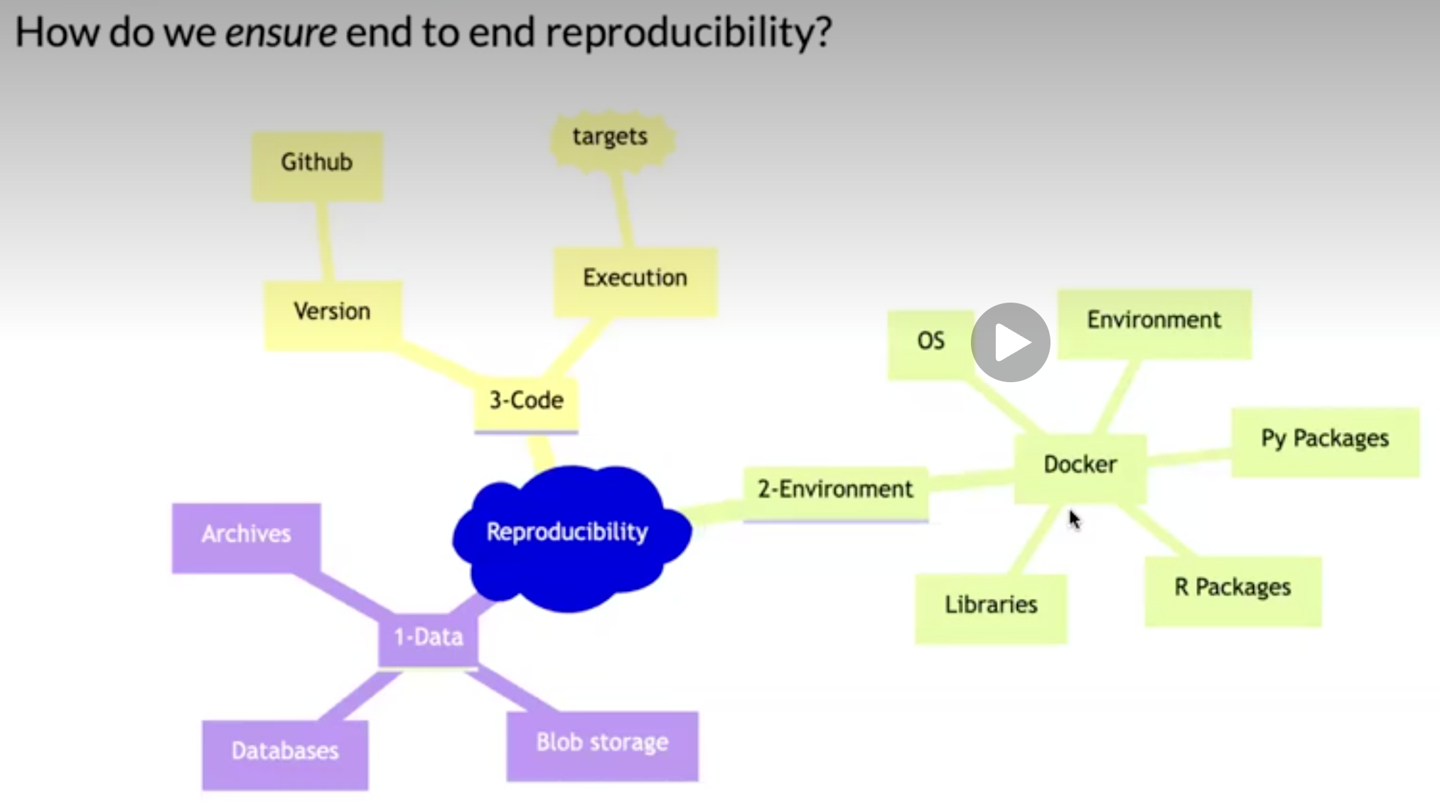
Follow the recording from the workshop while you are practicing: The power of {targets} package for reproducible data science

Notes on the recording

The full video is close to three hours long, but this includes breaks as well as the more advanced topics that are not mandatory (only the first 92 minutes, which includes several 10 min breaks is mandatory). Nevertheless, it is recommended to watch the full video (just watching part 4-7 for inspirational purposes without doing the exercises and without any expectation to fully grasp all the details).
RStudio is used in the recording. Please try to use Positron; however, feel free to revert to RStudio this time if following the instructions in one application while working in another feels overwhelming.
You may recognize some of the material from Part 3, as presented during the lecture

This practice is homework (no dedicated computer session is targeting targets but you should use at least some components of it in a later project, so you should practice the basics now)!

Motivational quotes

An article about computational science in a scientific publication is not the scholarship itself, it is merely advertising of the scholarship. The actual scholarship is the complete software development environment and the complete set of instructions which generated the figures. / Buckheit & Donoho

[It is important to have] a clear understanding of how data analysis was conducted when critical life and death decisions must be made. / Peng et al. 2021

Reproducible analysis

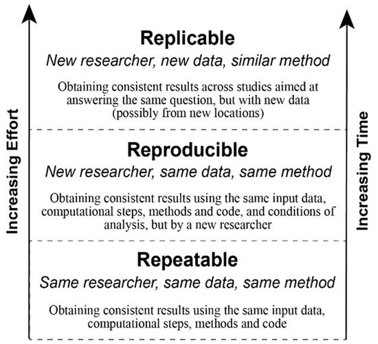
The definition of reproducible research generally consists of the following elements.

A published data analysis is reproducible if the analytic data sets and the computer code used to create the data analysis are made available to others for independent study and analysis

This is rather vague …

Why is this a problem?

Many, even simple, results depend on a precise record of procedures and processing and the order in which they occur.
Many statistical algorithms have many tuning parameters that can dramatically change the results if they are not inputted exactly the same way as was done by the original investigators.
If any of these myriad details are not properly recorded in the code, then there is a significant possibility that the results produced by others will differ from the original investigators’ results.

Recap folder structure

/.../my_project/
  ├── README.md        - project documentation
  ├── TODO             - what should be done next?
  ├── .git             - handled by git (hidden folder)
  ├── .gitignore       - used by git but your responsibility!
  ├── data/            - your data files (not under version control!)
      ├── cancer.csv 
      └── patients.qs 
  ├── R/               - your saved R functions
      ├── function1.R 
      └── function2.R
  ├── reports/
  └── _targets.R       - targets pipeline script

Pipeline

A pipeline is a computational workflow that does statistics, analytics, or data science.
A pipeline contains tasks to prepare datasets, run models, and summarize results for a business deliverable or research paper.
Pipeline tools coordinate the pieces of computationally demanding analysis projects.

Pipe operator

The simplest example of pipelines might be when you combine R code by the pipe operator (|> or %>%), which in turn is inspired by the pipe operator in Unix (|).

Long running processes

Imaigine you have nice R-scripts to take care of every step in your project
You have either one very very … very … long file or a bunch of files which you execute in order
It takes two weeks to run all scripts (not unrealistic for a big project!)
You report the result to your collaborators
They ask you to update a tiny detail somewhere in the middle of your workflow
You need to rerun everything (while screaming in frustration)!
This will repeat again and again until you finally
1. Lose your mind and quit your job
2. Adapt a more reproducible workflow

Steps-wise procedure

The default setting in R is to save the workspace to disk when you end the session
This is usually not recommended and therefore often disabled in for example RStudio
- (If you re-start your session at a later point you might have no idea how the restored objects relates to each other.)
You may still want to execute things in a more step-wise fashion
1. Convert big data files (.sas7bdat from SAS etc) to something more R-friendly
2. Perform some data management (select relevant columns and rows), cleaning, add calculated variables etc
3. Perform some exploratory data analysis (EDA) to get a better understanding of the data
4. Perform some statistical analysis
5. Report and visualize the results

Caching

If you perform each step in different script files, you might start each file with some input and end it with some output
The output from the previous script is used as input in the next script
save() and load() are standard but can be very slow for large objects
saveRDS() and loadRDS() use serialization and are nowadays much more efficient
qs2::qs_save() and qs2::qs_read() (or qs2::qd_save() and qs2::qd_read()) from the qs2 package are currently “state-of-the-art” (but things tend to change quickly)

Benchmarking

Single-threaded

Algorithm	Compression	Save Time (s)	Read Time (s)
qs2	7.96	13.4	50.4
qdata	8.45	10.5	34.8
base::serialize	1.1	8.87	51.4
saveRDS	8.68	107	63.7
fst	2.59	5.09	46.3
parquet	8.29	20.3	38.4
qs (legacy)	7.97	9.13	48.1

Multi-threaded (8 threads)

Algorithm	Compression	Save Time (s)	Read Time (s)
qs2	7.96	3.79	48.1
qdata	8.45	1.98	33.1
fst	2.59	5.05	46.6
parquet	8.29	20.2	37.0
qs (legacy)	7.97	3.21	52.0

qs2, qdata and qs with compress_level = 3
parquet via the arrow package using zstd compression_level = 3
base::serialize with ascii = FALSE and xdr = FALSE

Datasets used

1000 genomes non-coding VCF 1000 genomes non-coding variants (2743 MB)
B-cell data B-cell mouse data, Greiff 2017 (1057 MB)
IP location IPV4 range data with location information (198 MB)
Netflix movie ratings Netflix ML prediction dataset (571 MB)

These datasets are openly licensed and represent a combination of numeric and text data across multiple domains. See inst/analysis/datasets.R on Github.

Who cares?

Imagine you work with data for the whole Swedish population (> 10 M people)
You have medical prescription data for everyone and lets say on average 20 prescriptions (since 2015) per person => 10 * 20 = 200 M rows of data
You are working in a secure environment were data is stored on a network server (no SSD drive)
The same environment is shared by 20 other researchers and you are all competing for the same bandwidth
It will get increasingly frustrating just to load and save the big files
You might need to wait for half an hour before you can start working 😩

Automated process

Instead of relying on individual R scripts, use a reproducible pipeline.
This is common practice in software development
- For example GNU Make is a build automation tool that automatically determines which parts of a program need to be rebuilt and executes the necessary commands based on rules defined in a Makefile.
Iteration during project development (which is equally relevant for a health data project), will be much faster and reliable.
Caching as described above is automated and you only need to read/write files to disk/network storage when actually needed.

Alternative solutions

GNU Make with R
rmake creates and maintains a build process for complex analytic tasks. The package allows easy generation of a Makefile for the (GNU) ‘make’ tool
drake was the first more established R-oriented alternative
targets is the currently most developed and used alternative
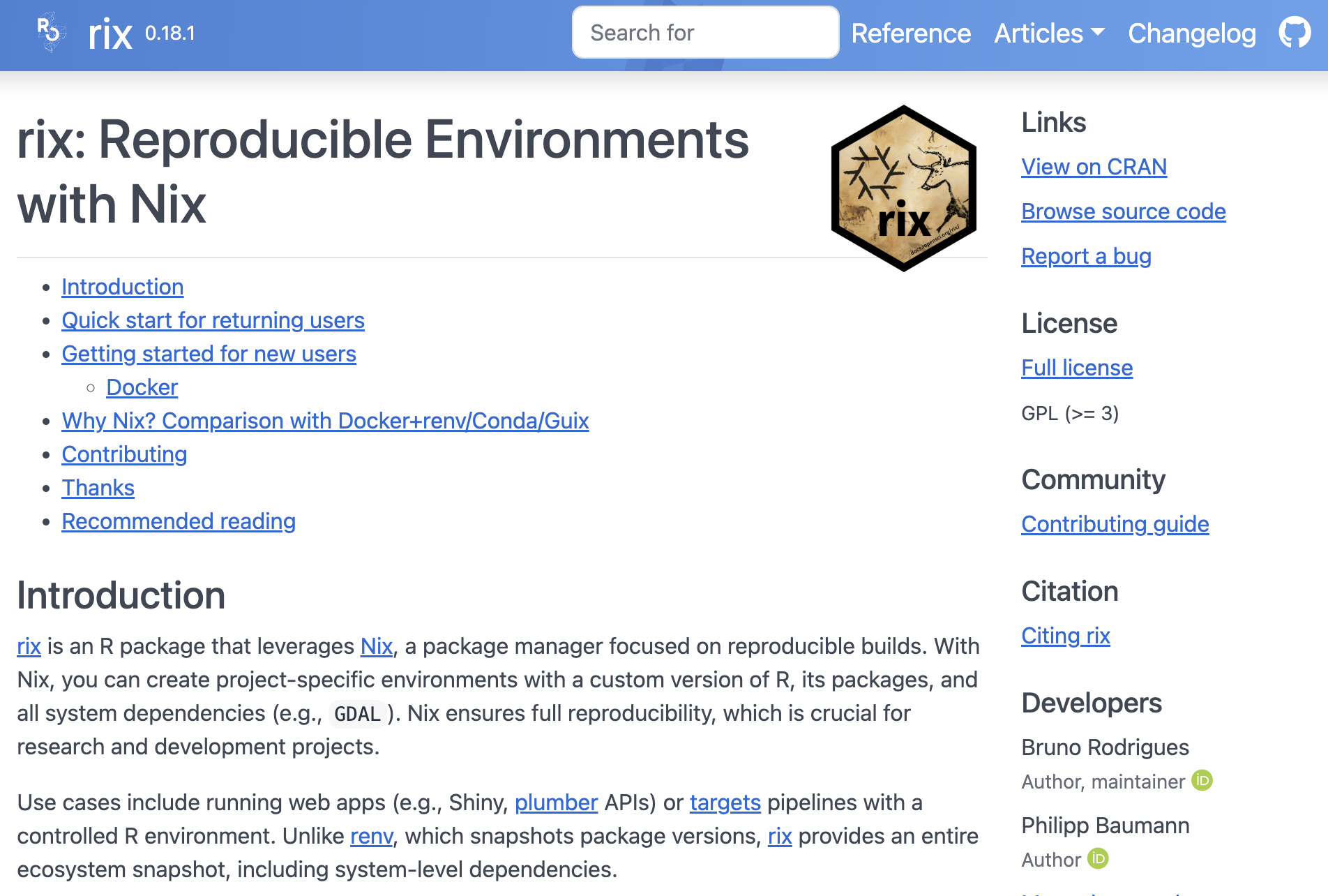
rixpress might be a rising star (at least if you are combining R and Python; polyglot)?

We will use targets in this course!

targets

The {targets} package is a Make-like pipeline tool for statistics and data science in R.
The package skips costly runtime for tasks that are already up to date, orchestrates the necessary computation with implicit parallel computing, and abstracts files as R objects.
If all the current output matches the current upstream code and data, then the whole pipeline is up to date, and the results are more trustworthy than otherwise.
The tasks themselves are called “targets”, and they run the functions and return R objects.
The targets package orchestrates the targets and stores the output objects to make your pipeline efficient, painless (well … hopefully relatively so …), and reproducible.

Example

Data: survey data collected by the US National Center for Health Statistics (NCHS) which has conducted a series of health and nutrition surveys since the early 1960’s. Since 1999 approximately 5,000 individuals of all ages are interviewed in their homes every year and complete the health examination component of the survey.

Question: Is there any association between Gender and BMI?

# pak::pkg_install("NHANES")
str(NHANES::NHANES)

Classes 'tbl_df', 'tbl' and 'data.frame':   10000 obs. of  76 variables:
 $ ID              : int  51624 51624 51624 51625 51630 51638 51646 51647 51647 51647 ...
 $ SurveyYr        : Factor w/ 2 levels "2009_10","2011_12": 1 1 1 1 1 1 1 1 1 1 ...
 $ Gender          : Factor w/ 2 levels "female","male": 2 2 2 2 1 2 2 1 1 1 ...
 $ Age             : int  34 34 34 4 49 9 8 45 45 45 ...
 $ AgeDecade       : Factor w/ 8 levels " 0-9"," 10-19",..: 4 4 4 1 5 1 1 5 5 5 ...
 $ AgeMonths       : int  409 409 409 49 596 115 101 541 541 541 ...
 $ Race1           : Factor w/ 5 levels "Black","Hispanic",..: 4 4 4 5 4 4 4 4 4 4 ...
 $ Race3           : Factor w/ 6 levels "Asian","Black",..: NA NA NA NA NA NA NA NA NA NA ...
 $ Education       : Factor w/ 5 levels "8th Grade","9 - 11th Grade",..: 3 3 3 NA 4 NA NA 5 5 5 ...
 $ MaritalStatus   : Factor w/ 6 levels "Divorced","LivePartner",..: 3 3 3 NA 2 NA NA 3 3 3 ...
 $ HHIncome        : Factor w/ 12 levels " 0-4999"," 5000-9999",..: 6 6 6 5 7 11 9 11 11 11 ...
 $ HHIncomeMid     : int  30000 30000 30000 22500 40000 87500 60000 87500 87500 87500 ...
 $ Poverty         : num  1.36 1.36 1.36 1.07 1.91 1.84 2.33 5 5 5 ...
 $ HomeRooms       : int  6 6 6 9 5 6 7 6 6 6 ...
 $ HomeOwn         : Factor w/ 3 levels "Own","Rent","Other": 1 1 1 1 2 2 1 1 1 1 ...
 $ Work            : Factor w/ 3 levels "Looking","NotWorking",..: 2 2 2 NA 2 NA NA 3 3 3 ...
 $ Weight          : num  87.4 87.4 87.4 17 86.7 29.8 35.2 75.7 75.7 75.7 ...
 $ Length          : num  NA NA NA NA NA NA NA NA NA NA ...
 $ HeadCirc        : num  NA NA NA NA NA NA NA NA NA NA ...
 $ Height          : num  165 165 165 105 168 ...
 $ BMI             : num  32.2 32.2 32.2 15.3 30.6 ...
 $ BMICatUnder20yrs: Factor w/ 4 levels "UnderWeight",..: NA NA NA NA NA NA NA NA NA NA ...
 $ BMI_WHO         : Factor w/ 4 levels "12.0_18.5","18.5_to_24.9",..: 4 4 4 1 4 1 2 3 3 3 ...
 $ Pulse           : int  70 70 70 NA 86 82 72 62 62 62 ...
 $ BPSysAve        : int  113 113 113 NA 112 86 107 118 118 118 ...
 $ BPDiaAve        : int  85 85 85 NA 75 47 37 64 64 64 ...
 $ BPSys1          : int  114 114 114 NA 118 84 114 106 106 106 ...
 $ BPDia1          : int  88 88 88 NA 82 50 46 62 62 62 ...
 $ BPSys2          : int  114 114 114 NA 108 84 108 118 118 118 ...
 $ BPDia2          : int  88 88 88 NA 74 50 36 68 68 68 ...
 $ BPSys3          : int  112 112 112 NA 116 88 106 118 118 118 ...
 $ BPDia3          : int  82 82 82 NA 76 44 38 60 60 60 ...
 $ Testosterone    : num  NA NA NA NA NA NA NA NA NA NA ...
 $ DirectChol      : num  1.29 1.29 1.29 NA 1.16 1.34 1.55 2.12 2.12 2.12 ...
 $ TotChol         : num  3.49 3.49 3.49 NA 6.7 4.86 4.09 5.82 5.82 5.82 ...
 $ UrineVol1       : int  352 352 352 NA 77 123 238 106 106 106 ...
 $ UrineFlow1      : num  NA NA NA NA 0.094 ...
 $ UrineVol2       : int  NA NA NA NA NA NA NA NA NA NA ...
 $ UrineFlow2      : num  NA NA NA NA NA NA NA NA NA NA ...
 $ Diabetes        : Factor w/ 2 levels "No","Yes": 1 1 1 1 1 1 1 1 1 1 ...
 $ DiabetesAge     : int  NA NA NA NA NA NA NA NA NA NA ...
 $ HealthGen       : Factor w/ 5 levels "Excellent","Vgood",..: 3 3 3 NA 3 NA NA 2 2 2 ...
 $ DaysPhysHlthBad : int  0 0 0 NA 0 NA NA 0 0 0 ...
 $ DaysMentHlthBad : int  15 15 15 NA 10 NA NA 3 3 3 ...
 $ LittleInterest  : Factor w/ 3 levels "None","Several",..: 3 3 3 NA 2 NA NA 1 1 1 ...
 $ Depressed       : Factor w/ 3 levels "None","Several",..: 2 2 2 NA 2 NA NA 1 1 1 ...
 $ nPregnancies    : int  NA NA NA NA 2 NA NA 1 1 1 ...
 $ nBabies         : int  NA NA NA NA 2 NA NA NA NA NA ...
 $ Age1stBaby      : int  NA NA NA NA 27 NA NA NA NA NA ...
 $ SleepHrsNight   : int  4 4 4 NA 8 NA NA 8 8 8 ...
 $ SleepTrouble    : Factor w/ 2 levels "No","Yes": 2 2 2 NA 2 NA NA 1 1 1 ...
 $ PhysActive      : Factor w/ 2 levels "No","Yes": 1 1 1 NA 1 NA NA 2 2 2 ...
 $ PhysActiveDays  : int  NA NA NA NA NA NA NA 5 5 5 ...
 $ TVHrsDay        : Factor w/ 7 levels "0_hrs","0_to_1_hr",..: NA NA NA NA NA NA NA NA NA NA ...
 $ CompHrsDay      : Factor w/ 7 levels "0_hrs","0_to_1_hr",..: NA NA NA NA NA NA NA NA NA NA ...
 $ TVHrsDayChild   : int  NA NA NA 4 NA 5 1 NA NA NA ...
 $ CompHrsDayChild : int  NA NA NA 1 NA 0 6 NA NA NA ...
 $ Alcohol12PlusYr : Factor w/ 2 levels "No","Yes": 2 2 2 NA 2 NA NA 2 2 2 ...
 $ AlcoholDay      : int  NA NA NA NA 2 NA NA 3 3 3 ...
 $ AlcoholYear     : int  0 0 0 NA 20 NA NA 52 52 52 ...
 $ SmokeNow        : Factor w/ 2 levels "No","Yes": 1 1 1 NA 2 NA NA NA NA NA ...
 $ Smoke100        : Factor w/ 2 levels "No","Yes": 2 2 2 NA 2 NA NA 1 1 1 ...
 $ Smoke100n       : Factor w/ 2 levels "Non-Smoker","Smoker": 2 2 2 NA 2 NA NA 1 1 1 ...
 $ SmokeAge        : int  18 18 18 NA 38 NA NA NA NA NA ...
 $ Marijuana       : Factor w/ 2 levels "No","Yes": 2 2 2 NA 2 NA NA 2 2 2 ...
 $ AgeFirstMarij   : int  17 17 17 NA 18 NA NA 13 13 13 ...
 $ RegularMarij    : Factor w/ 2 levels "No","Yes": 1 1 1 NA 1 NA NA 1 1 1 ...
 $ AgeRegMarij     : int  NA NA NA NA NA NA NA NA NA NA ...
 $ HardDrugs       : Factor w/ 2 levels "No","Yes": 2 2 2 NA 2 NA NA 1 1 1 ...
 $ SexEver         : Factor w/ 2 levels "No","Yes": 2 2 2 NA 2 NA NA 2 2 2 ...
 $ SexAge          : int  16 16 16 NA 12 NA NA 13 13 13 ...
 $ SexNumPartnLife : int  8 8 8 NA 10 NA NA 20 20 20 ...
 $ SexNumPartYear  : int  1 1 1 NA 1 NA NA 0 0 0 ...
 $ SameSex         : Factor w/ 2 levels "No","Yes": 1 1 1 NA 2 NA NA 2 2 2 ...
 $ SexOrientation  : Factor w/ 3 levels "Bisexual","Heterosexual",..: 2 2 2 NA 2 NA NA 1 1 1 ...
 $ PregnantNow     : Factor w/ 3 levels "Yes","No","Unknown": NA NA NA NA NA NA NA NA NA NA ...

R script

A normal R script might look like:

# pak::pkg_install("NHANES")
library(tidyverse)

df <- as_tibble(NHANES::NHANES)
tbl <- count(df, Gender)
tst <- t.test(BMI ~ Gender, df)
gg <- ggplot(df, aes(BMI, color = Gender)) + geom_density()

You must run the script in order (but might not always do that during the initial “trial and error” process … if so, confusion will later arise)!
objects df, tbl and tst only lives in the active session
- No problem in this example
- but working with big and complex data might introduce long-running processes => time consuming!

Results


    Welch Two Sample t-test

data:  BMI by Gender
t = 1.4981, df = 9452.6, p-value = 0.1341
alternative hypothesis: true difference in means between group female and group male is not equal to 0
95 percent confidence interval:
 -0.06939849  0.51940903
sample estimates:
mean in group female   mean in group male 
            26.77208             26.54707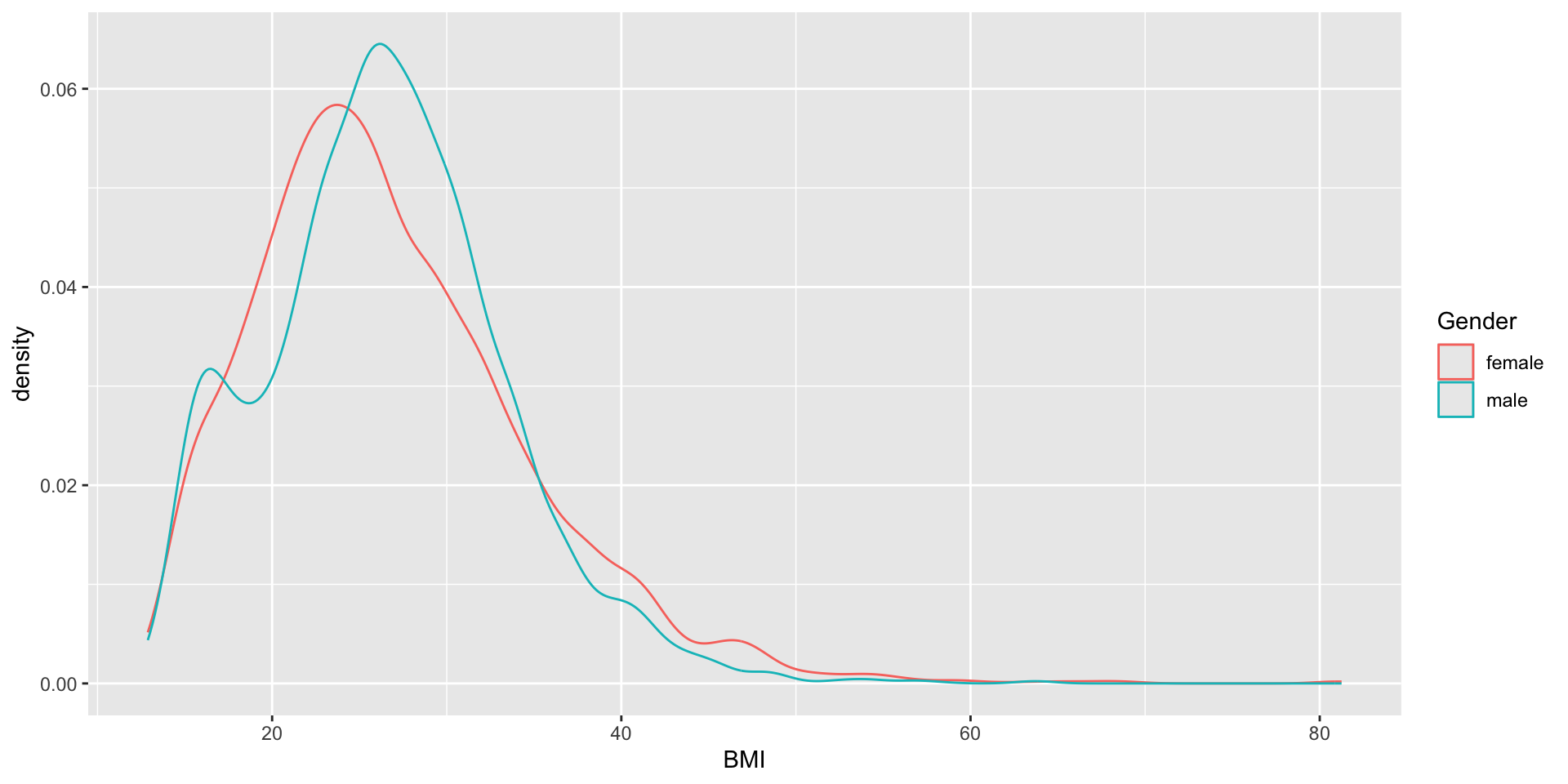

Figure and R output

You should see a figure and some R output on this slide. I just notice it doesn’t show on my phone when viewing the slides, so if you don’t see it, you might try another browser etc (it seems to render correct in the handouts however).

Pipeline

Define steps in your analysis as targets
Define dependencies between targets
Automatically track changes and rerun only necessary parts

Why?

You do not want to rerun everything all the time!
You want to keep track of what you have done
You want to be able to reproduce your results later
You want to share your workflow with others

target

Reformulate from ordinary object assignment:

df <- as_tibble(NHANES::NHANES)

to a target

library(targets)
tar_target(df, as_tibble(NHANES::NHANES))

<tar_stem> 
  name: df 
  description:  
  command:
    as_tibble(NHANES::NHANES) 
  format: rds 
  repository: local 
  iteration method: vector 
  error mode: stop 
  memory mode: auto 
  storage mode: worker 
  retrieval mode: auto 
  deployment mode: worker 
  priority: 0 
  resources:
    list() 
  cue:
    seed: TRUE
    file: TRUE
    iteration: TRUE
    repository: TRUE
    format: TRUE
    depend: TRUE
    command: TRUE
    mode: thorough 
  packages:
    targets
    lubridate
    forcats
    stringr
    dplyr
    purrr
    readr
    tidyr
    tibble
    ggplot2
    tidyverse
    stats
    graphics
    grDevices
    utils
    datasets
    methods
    base 
  library:
    NULL

Put all targets in a list

list(
  tar_target(df, as_tibble(NHANES::NHANES)),
  tar_target(tbl, count(df, Species)),
  tar_target(tst, t.test(BMI ~ Gender, df)),
  tar_target(gg, {
    ggplot(df, aes(BMI, color = Gender)) + geom_density()
  })
)

`_targets.R` file

Put that list into a file _targets.R together with some additional code:

library(targets)
tar_source() # Source all scripts with functions stored in R folder
tar_option_set(
  # Specify all needed packages here
  # NOTE! They will not be available in the interactive R-session
  # so you might load them above as well to avoid confusion
  packages = c("tidyverse"),
  # Format used for caching (qs which is actually qs2 is best for big data)
  format = "qs",
  # Additional settings ...
  seed = 123
)

list(
  tar_target(df, as_tibble(NHANES::NHANES)),
  tar_target(tbl, count(df, Species)),
  tar_target(tst, t.test(BMI ~ Gender, df)),
  tar_target(gg, {
    ggplot(df, aes(BMI, color = Gender)) + geom_density()
  })
)

Benefits

execute the whole project by tar_make()
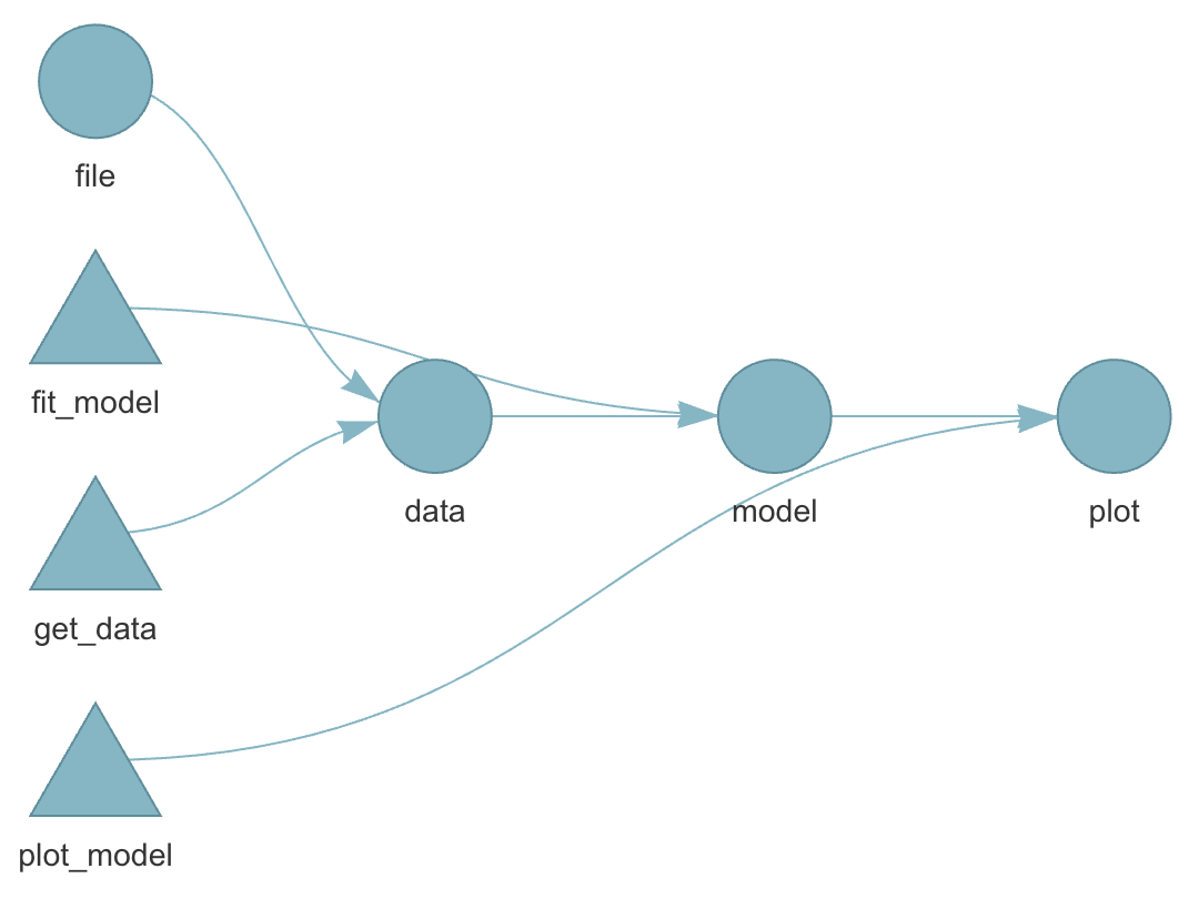
intermediate steps are cached and cached objects retrieved by tar_load() or tar_read()
dependency among individual steps can be visualized: tar_visnetwork()

Dependency graph

Live show

cd
git clone https://github.com/STA220/targets.git
cd targets
positron .

Or perform those steps from within Positron.

R-versions

Imagine you finish your research project and you submit a manuscript to a journal
The journal comes back one year later (they didn’t have time until know) and one reviewer ask you to double check some steps of the analysis
You make some modifications and rerun your pipelines.
But it doesn’t work!
Half a year ago you updated your R installation and a week ago all of your installed packages.
- One package was retired from CRAN (could happen even though there was nothing wrong with the package when you used it … maybe the maintainer just didn’t have time or energy to keep maintaining it)
- One package has deprecated one of the functions you previously used
- On package has redesigned the output format from a specific function you used
😱

Pros and cons

It is always a good idea to be able to reproduce exactly what you did!
But if you never update you might miss essential bug fixes!
If your results change, how can you know which version was the most accurate?

Best practice (I guess) is to rerun the analysis both with the frozen versions and with the most up-to-date versions of the packages … because you have all the time in the world and nothing more important to do … right … 😂

Different operating systems

R should behave similar on different operating systems.
Exceptions nevertheless exist!
- parallel::mclapply() behaves differently on Windows compared to Unix-like systems because Windows does not support forked processes.
- sort(c("ä", "a", "z")) might differ due to locale settings
- Earlier versions of R relied on system-specific native encoding (notably on Windows), whereas modern versions (R ≥ 4.2) use UTF-8 as the default across platforms.

Combining all?

you could very well use both targets + renv + git + GitHub etc
At some point you might start to wonder whether you are a medical statistician or a software developer … and the more complex/esoteric tools you use, the more difficult it might be to collaborate with others
Try to find some middle ground … but always be open to new ideas!

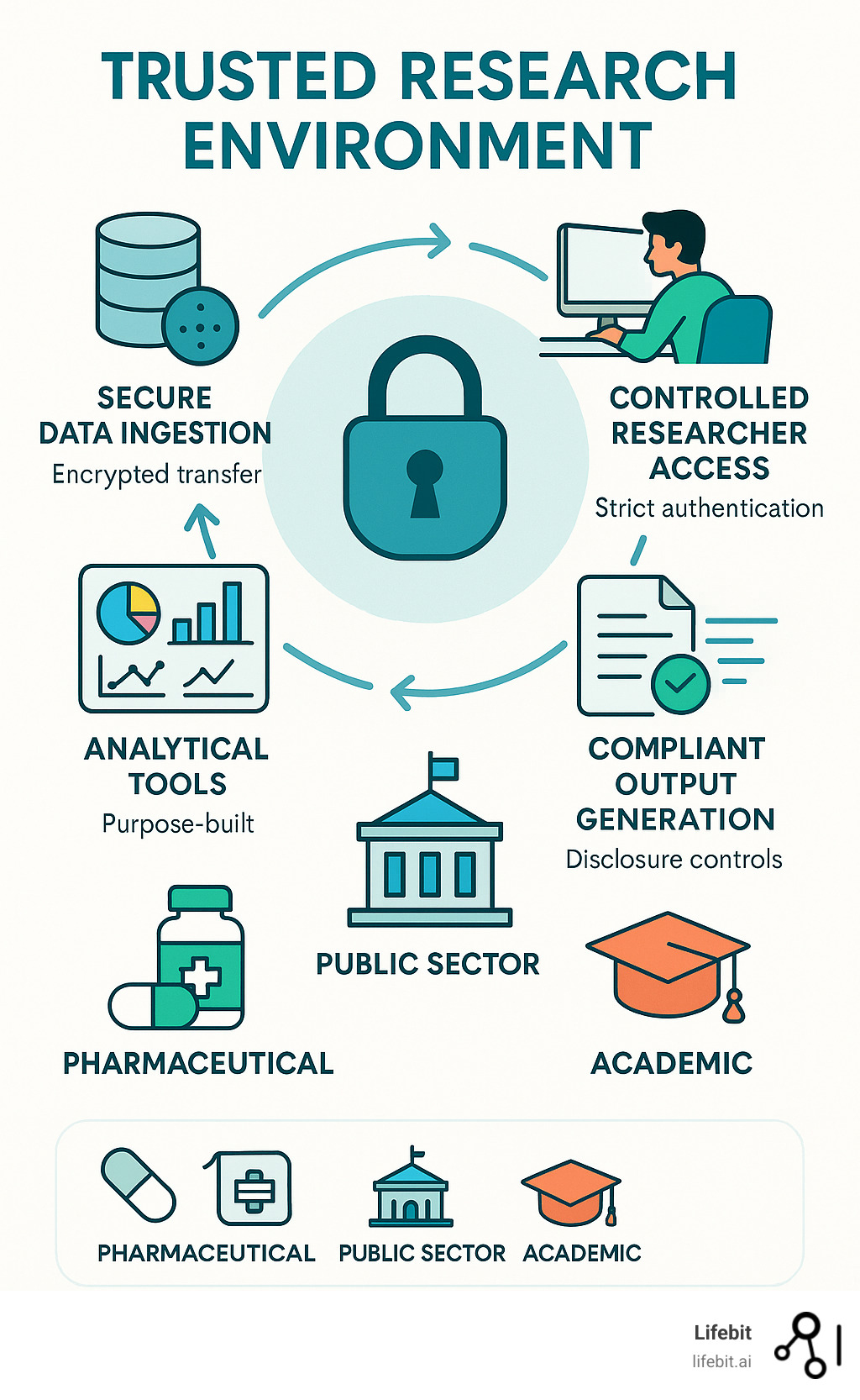
TRE

Historically: centralized data on mainframe computer
More recently: working with data locally (desktop/laptop)
- Full volume encryption (BitLocker on Windows, FileVault on Mac etc)
- Possible to work off-line (trains, flights etc)
- Backups! Backups!!! BACKUPS!!!
- Usually only password protected and no logging of of activities
- Sometimes admin user (sometimes not)
Nowadays: (Different names, same concept) Secure Research Envoronemnt (SRE), Trusted Research Envoronment (TRE), Secure Data Environment (SDE), Data Clean Room, Data Safe Havens, …

In practice

Connect through VPN
2-factor authentication (BankID common in Sweden)
Often by Remote Desktop (to access a Windows virtual desktop)
Sometimes a containerized Linux setup for R/RStudio etc accessed through a web browser (from within the virtual Windows machine)
Limited internet access from within the environment (maybe possible to install CRAN-packages tied to a certain historical snapshot but not the latest released/developed versions).
Data import and exports goes through administrator
Pros: Secure, centralized backups, possibility to scale/share large computing resources (CPU, RAM, GPU etc), less dependent on individual computer (laptop), might aid collaboration
Cons: needs internet connection, restrictions on what software (packages) to use, difficult to export results and/or import script files etc, mentally exhausting to use for example a Mac Keyboard when working in Windows, can be expensive (pay per clock-cycle of CPU usage etc instead of simply purchasing a computer once).

Baker, Monya. 2016. “1,500 Scientists Lift the Lid on Reproducibility.” Nature 533 (7604): 452–54. https://doi.org/10.1038/533452a.

Kavianpour, Sanaz, James Sutherland, Esma Mansouri-Benssassi, Natalie Coull, and Emily Jefferson. 2022. “Next-Generation Capabilities in Trusted Research Environments: Interview Study.” Journal of Medical Internet Research 24 (9): e33720. https://doi.org/10.2196/33720.

Nguyen, Andrew. 2022. Hands-on healthcare data: taming the complexity of real-world data. First edition. Beijing Boston Farnham Sebastopol Tokyo: O’Reilly.

Oliveira Andrade, Rodrigo de. 2025. “Huge Reproducibility Project Fails to Validate Dozens of Biomedical Studies.” Nature 641 (8062): 293–94. https://doi.org/10.1038/d41586-025-01266-x.

Peng, Roger D., and Stephanie C. Hicks. 2021. “Reproducible Research: A Retrospective.” Annual Review of Public Health 42 (Volume 42, 2021): 79–93. https://doi.org/10.1146/annurev-publhealth-012420-105110.

EL5: Reproducibility

Reading

Practice

Motivational quotes

Reproducible analysis

Why is this a problem?

Recap folder structure

Pipeline

Long running processes

Steps-wise procedure

Caching

Benchmarking

Single-threaded

Multi-threaded (8 threads)

Who cares?

Automated process

Alternative solutions

targets

Example

R script

Results

Pipeline

Why?

target

Put all targets in a list

_targets.R file

Benefits

Dependency graph

Live show

R-versions

Pros and cons

Different operating systems

Combining all?

TRE

In practice

`_targets.R` file