EL9: Documentation

Quarto

Reading

(Wickham, Çetinkaya-Rundel, and Grolemund, n.d., ch. 28-29) introduces Quarto with good examples

For reference

quarto.org

Levels of documentation

Documentation can exist at several levels in a project.

Code level
- scripts (comments, e.g. # clean data and merge cohorts)
- functions (Roxygen2 documentation)
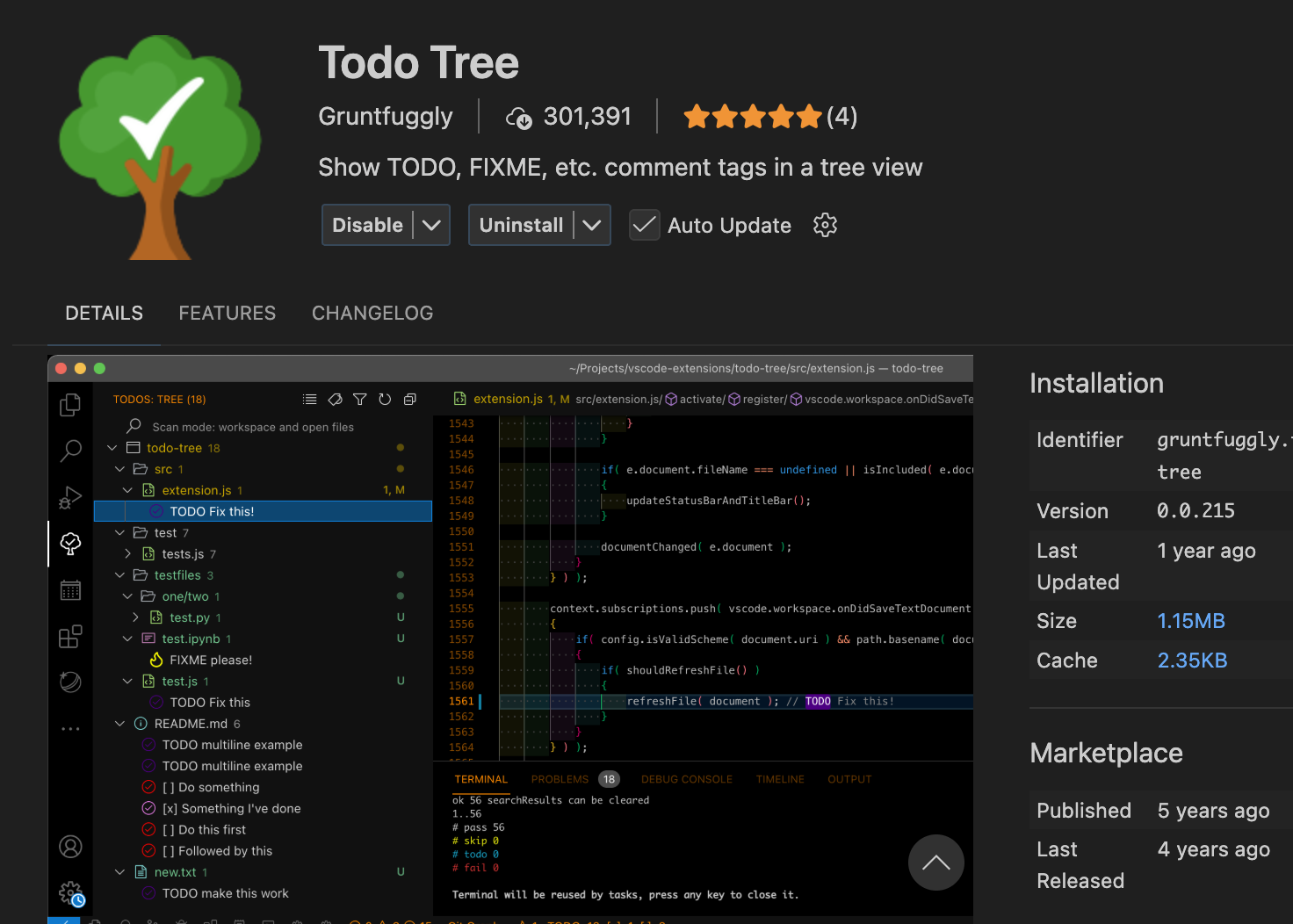
- notes and reminders (e.g. # TODO:)
Project level
- README.md
- (GitHub repos may also have a wiki or a polished website)
Output level
- figures and tables
- reports (PDF / HTML)
- presentations (slides)

Code level

Documenting R scripts

Use Air for better formatting of the R code itself (will format the code according to best practice for readability and collaboration)
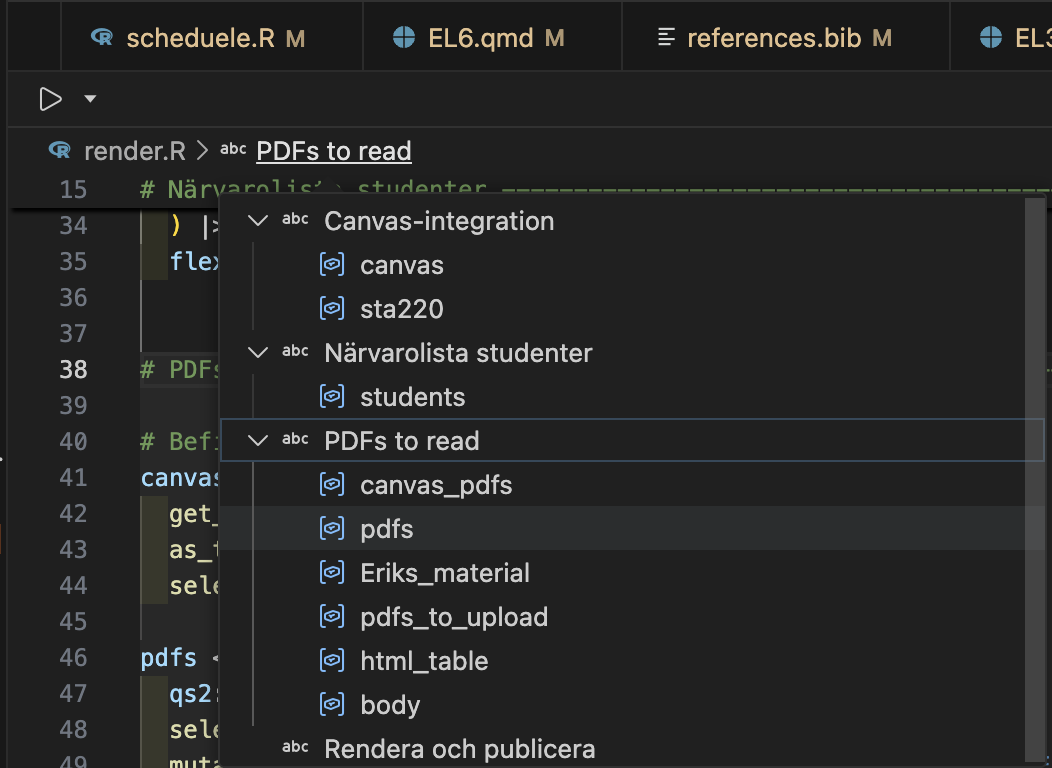
Section labels by Shift + Ctrl/Cmd + R in Positron (and RStudio)
Easiest way to aid navigation to R scripts

# My section heading -----------------------------------------------------

Individual scripts

As soon as you distribute an individual R script from a bigger project (by e-mail or as a printed copy) some context would get lost.
The commentr package is designed to maintain such context
- remotes::install_bitbucket("cancercentrum/commentr")

commentr::header_comment(
  "My nice script",
  "Bla bla bla ...",
  "Erik Bülow",
  "xxx@yyy.zzz",
  "John Doe"
)


###########################################################################
#                                                                         #
# Purpose:       My nice script                                           #
#                                                                         #
# Author:        Erik Bülow                                               #
# Contact:       xxx@yyy.zzz                                              #
# Client:        John Doe                                                 #
#                                                                         #
# Code created:  2026-03-20                                               #
# Last updated:  2026-03-20                                               #
# Source:        /Users/xbuler/STA220/documentation                       #
#                                                                         #
# Comment:       Bla bla bla ...                                          #
#                                                                         #
###########################################################################

# TODO: Change this to something better:
1 + 2

Documenting R functions

What does this function do?

hello <- function(who = "world") {
  sprintf("Hello %s!", who)
}

#' Say hello
#'
#' Create a simple greeting. If no name is provided, the function
#' returns a greeting to the world.
#'
#' @param who A character vector giving the name(s) of the person or
#'   object to greet. If missing, the greeting defaults to `"world"`.
#'
#' @return A character vector of the same length as `who` containing
#'   greeting messages.
#'
#' @examples
#' hello()
#' hello("you")
#' hello(c("Alice", "Bob"))
hello <- function(who = "world") {
  sprintf("Hello %s!", who)
}

There is a standardized syntax to document R functions
You should be able to click a small light bulb (💡) to insert a sceleton when writing your function
The same syntax is used within modern R packages
- but it is useful even within your own projects
roxygen2 is a package used for package documentation but it also has a great manual for documenteing functions in general

Project level

Documenting a project

You have a README.md file within your git repository
It can contain plain text without any formatting
It will be displayed up-front in GitHub
You can also include formatting!
It will be nicely rendered on GitHub or elsewhere

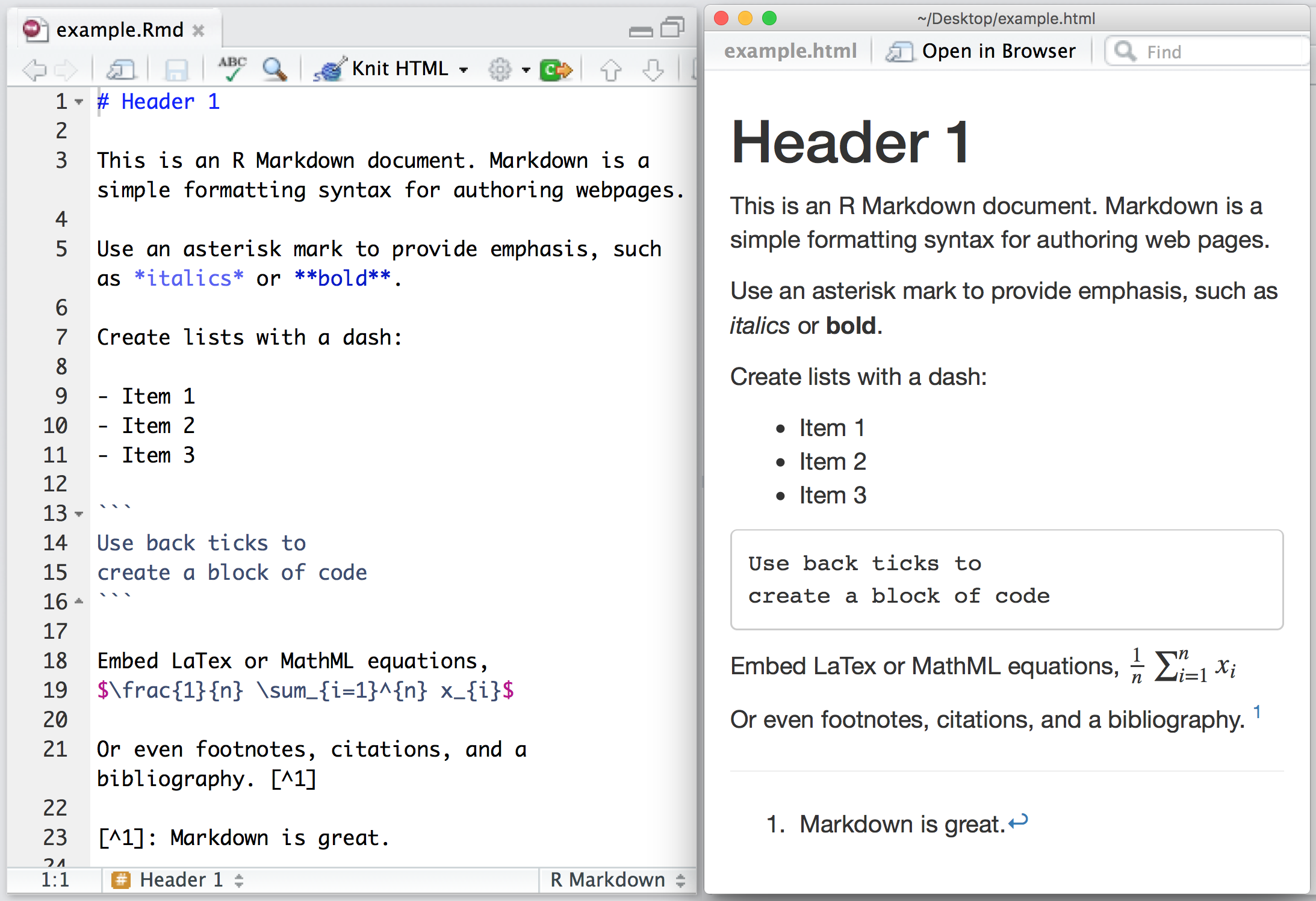
Basic formatting

What you want	Markdown syntax	Result
Heading	`# Heading`	Heading
Italic	`text`	text
Bold	`text`	text
Inline code	`code`	`code`
Link	`[text](https://example.com)`	text
Bullet list	`- item`	• item
Numbered list	`1. item`	1. item

Comment or heading

# is used for comments in R files and within R blocks but for headings in .md and .qmd files!

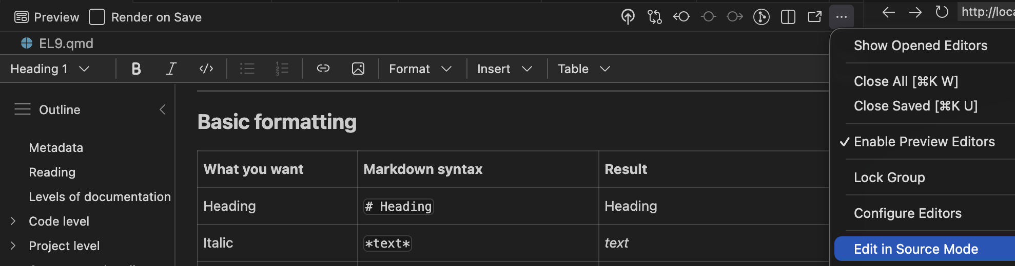
Visual mode

Instead of editing the source code, you may also use the “visual editor” in Positron:

Warning

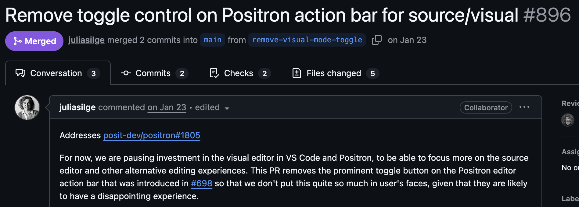
Use both?

Personally, I do most editing in source mode (better for the R chunks), but I find it much easier to include references/citations and to paste in external figures in using the visual mode.

Reproducible Workflows

Modern biostatistics projects rarely involve only statistics.

data cleaning and preprocessing
statistical modelling
visualisation
interpretation of results
reporting and documentation

A good workflow should make it possible to combine all of these steps in one place.

Output level

What?

Quarto is a publishing system for scientific and technical documents.

It allows you to combine:

text
R code
statistical results
tables and figures

in a single workflow.

This makes it easier to create reproducible statistical reports.

Why?

In many projects people work with:

R scripts for analysis 🥳
Word documents for reporting 😱
PowerPoint slides for presentations 😱

This separation often leads to:

copy–paste errors 🥴
outdated figures 👎
results that cannot easily be reproduced 🤯

Quarto helps avoid these problems!

Reproducible analysis

In a Quarto document you can:

write the explanation of your analysis
include the R code used
generate figures and tables automatically
update everything by re-running the document

If the data or model changes, the entire report can be regenerated automatically.
It is widely used in data science, epidemiology and biostatistics.
Integrated in Positron and developed by Posit PBC

Used in three ways

For communicating to decision-makers, who want to focus on the conclusions, not the code behind the analysis.
For collaborating with collegues (including future you!), who are interested in both your conclusions, and how you reached them (i.e. the code).
As an environment in which to do data science and statistics, as a modern-day lab notebook where you can capture not only what you did, but also what you were thinking.

A simple report

When you chose New > New File ... > Quarto document, the file will contain:

---
title: "Untitled"
format: html
---

This is a YAML header (Yet Another Markup Language)
Different output formats are available:
- html: can also be published online (Quartopub or GitHub pages)
- docx: Word document for collaborating with non-statisticians etc
- typst: PDF rendering (ever heard of \(\LaTeX\)? … This is the modern alternative!)
- revealjs: slide decks (you are looking at one!)
Can render to multiple formats at once!

This is the yaml header for this presentation:

---
title: "EL9: Documentation"
subtitle: "Quarto"
reading: "[@wickham, ch. 28-29]"
format:
  revealjs:
    theme: blood
    transition: fade
    slide-number: true
    css: styles.css
    smaller: true
    scrollable: true
    incremental: false
  typst:
    include-before-body:
      - text: |
          // Gör alla länkar tydliga i PDF: blå + understrukna
          #show link: set text(fill: rgb("1a5fb4"))
          #show link: underline
  docx: default
bibliography: references.bib
---

YAML structure

YAML uses indentation to represent structure.

Think of it like a tree.

format:
  html:
    code-fold: true

This corresponds to the structure:

format
└── html
    └── code-fold: true

If indentation is wrong?

format:
html:
  code-fold: true

Now Quarto interprets this as:

format
html
└── code-fold: true

This is not the intended structure, and the document may fail to render.

💡 Rule of thumb

use two spaces per level
never use tabs
when something fails, check indentation first

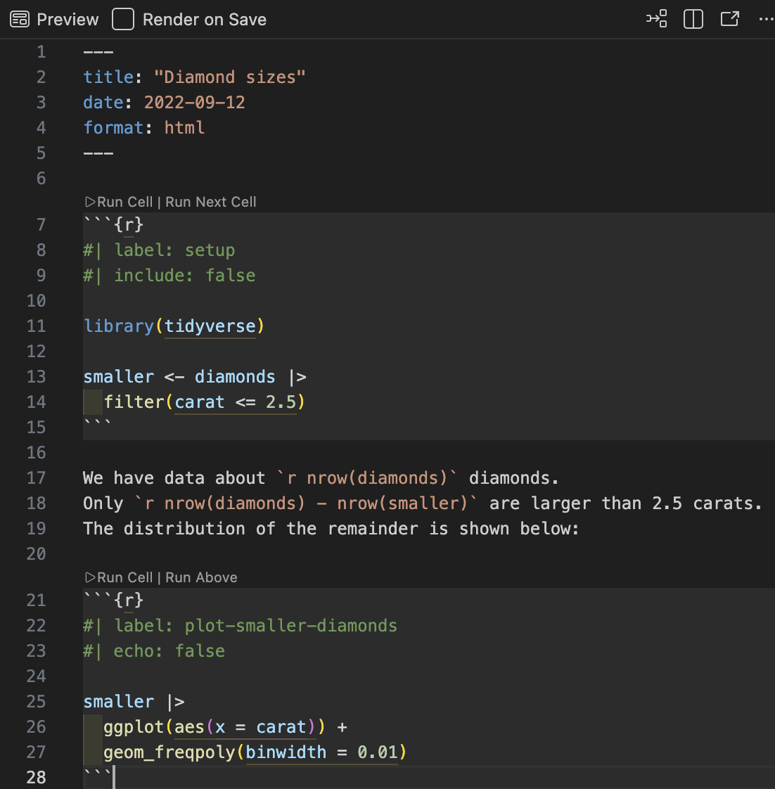
Three parts

Quarto documents have three parts:

An (optional) YAML header surrounded by ---s.
Chunks of R code surrounded by ```{r} and ```.

```{r}          ← chunk header
#| echo: false  ← options controlling the output
summary(x)      ← R code
```             ← end of chunk

Keybindings: Cmd + option + I (Mac) or Ctrl + Alt + I (Windows)

Text with markdown format

Order

Part 1 (YAML header) always comes first but 2 (code block) and 3 (Markdown text) are usually intermingled throughout the rest of the document.

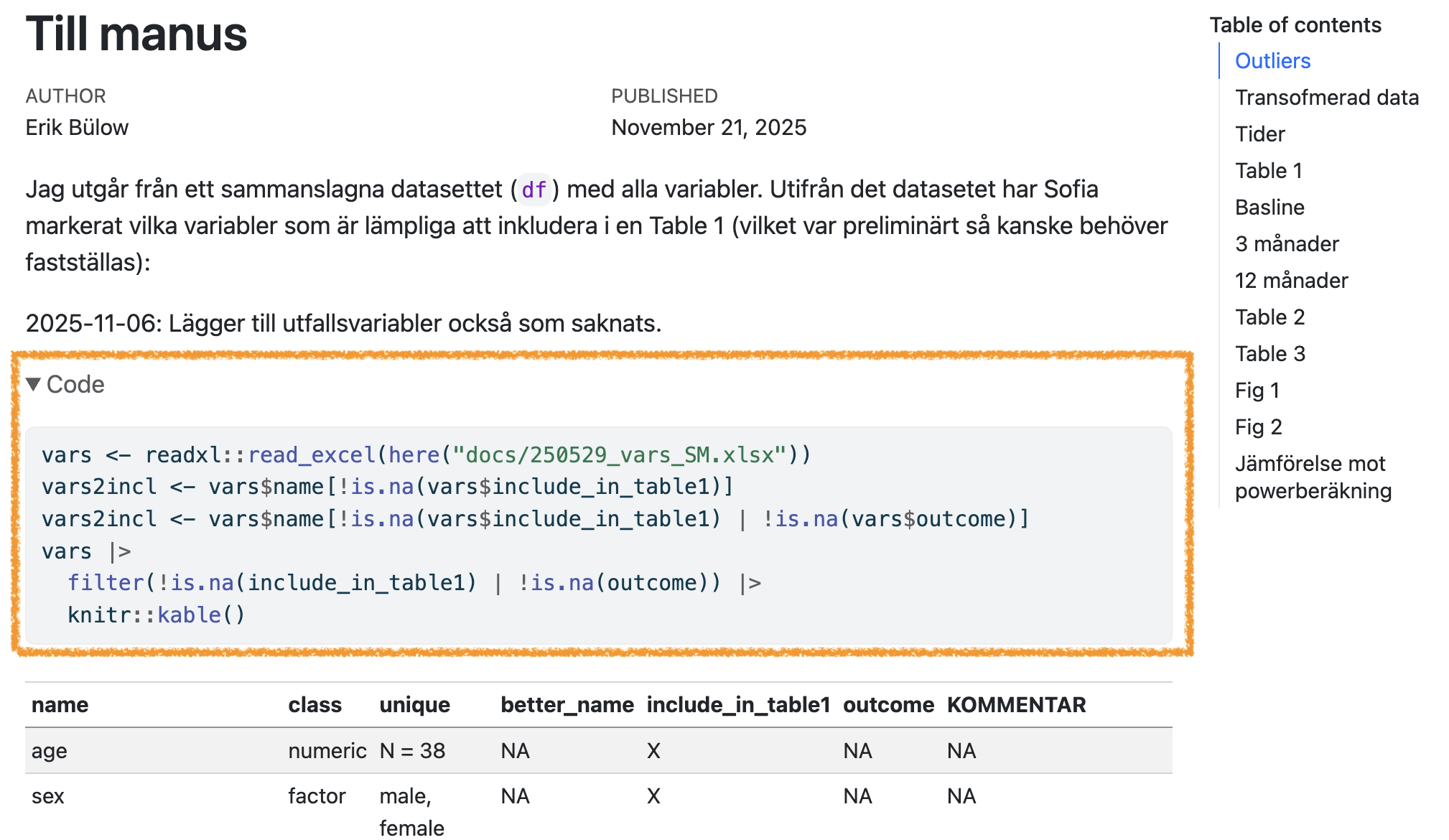
Inline code

Sometimes we want to insert small pieces of R output directly in the text.

This is called inline code.

Inline code will always just show the result of the call (not the code itself in the rendered document):

Todays date is `r Sys.Date()` and it is `r format(Sys.time(), format = "%H")`

Todys date is 2026-03-20 and it is 12 PM

To higlight with bold and italic:

Todays date is **`r Sys.Date()`** and it is *`r format(Sys.time(), format = "%I %p")`*

Todays date is 2026-03-20 and it is 12 PM

To publish

Decision makers, stake holders, friends or the public might not care about R. Disable R code (echoing the code itself), warnings and messages:

---
title: "Untitled"
format: html
execute:
  echo: false
  warning: false
  message: false
---

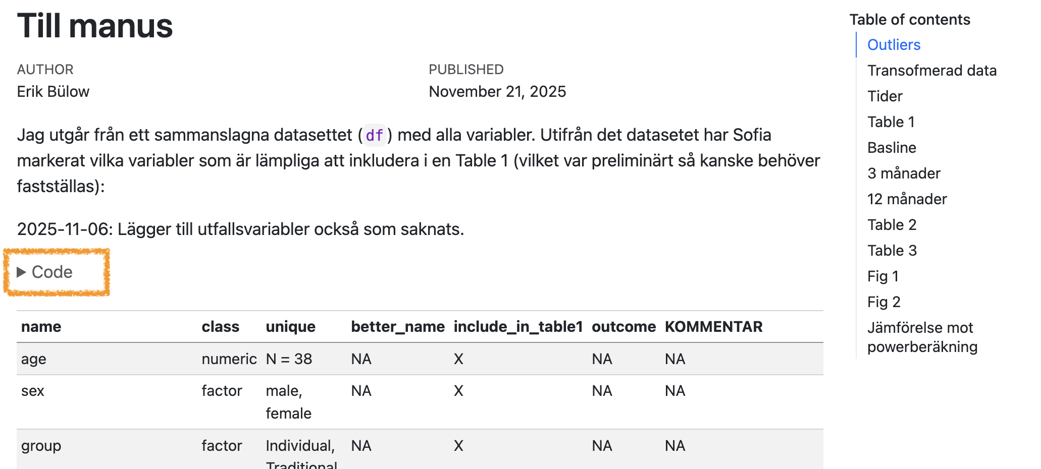
For collaborators

Might still care less about verbose R messages and warnings (they trust that you have already considered those)
May still need the underlaying R code for deeper understaing
Use code-fold

---
title: "Untitled"
format:
  html:
    code-fold: true
execute:
  warning: false
  message: false
---

This can also be set individually for each code chunk:

```{r}
#| echo: false
#| warning: false
#| message: true
message("will be muted!")
warning("will be ignored")
plot(something_beautiful, realy = TRUE)
```

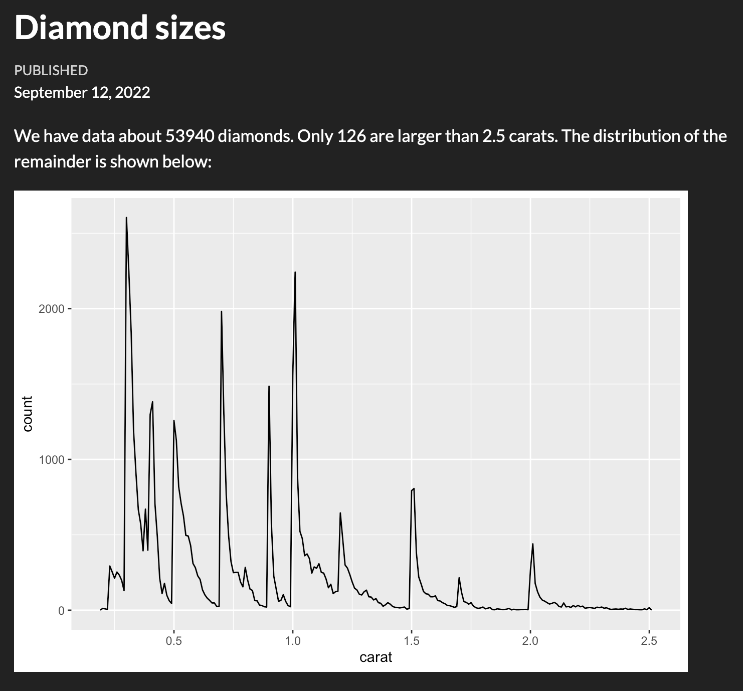
Figures

Figures are usualy displayed without problem (and you can adjust their size, add captions etc):

```{r}
#| fig-cap: This is origo!
plot(0, 0)
```

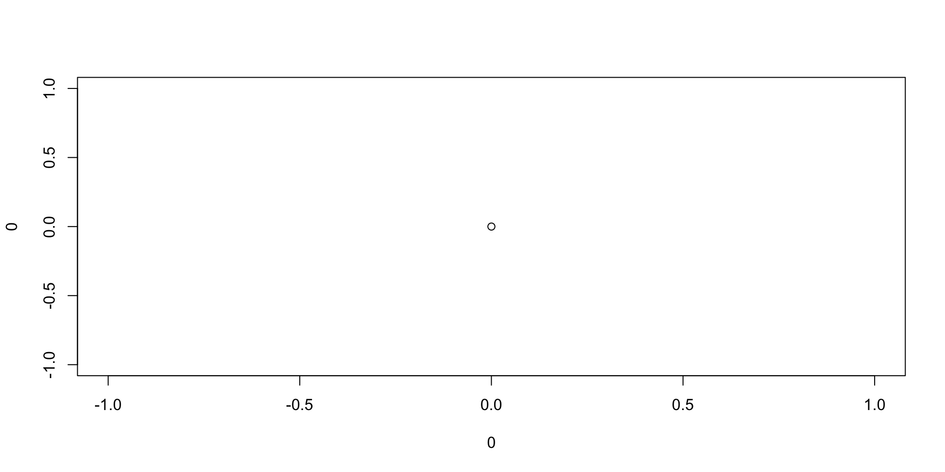
This is origo!

Tables

Just printing the R output might not look very nice:

head(iris)

  Sepal.Length Sepal.Width Petal.Length Petal.Width Species
1          5.1         3.5          1.4         0.2  setosa
2          4.9         3.0          1.4         0.2  setosa
3          4.7         3.2          1.3         0.2  setosa
4          4.6         3.1          1.5         0.2  setosa
5          5.0         3.6          1.4         0.2  setosa
6          5.4         3.9          1.7         0.4  setosa

Better with kable

The easiest way to make tibbles/data.frames/data.tables look nicer is with df-print: kable in the yaml header.

---
title: "Untitled"
format: html
df-print: kable
---

Or manually for individual outputs:

```{r}
#| tbl-cap: Some iris data
knitr::kable(head(iris))
```

Some iris data
Sepal.Length	Sepal.Width	Petal.Length	Petal.Width	Species
5.1	3.5	1.4	0.2	setosa
4.9	3.0	1.4	0.2	setosa
4.7	3.2	1.3	0.2	setosa
4.6	3.1	1.5	0.2	setosa
5.0	3.6	1.4	0.2	setosa
5.4	3.9	1.7	0.4	setosa

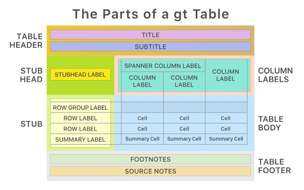
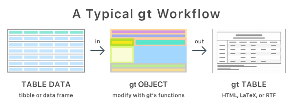
Best with gt

Very flexible
Publication ready
Package from Posit
flextable may be preferred instead if rendering Office documents (Word, PowerPoint)

gtsummary

gtsummary package build on top of {gt} to easily summarise datasets, regression models etc

```{r}
gtsummary::tbl_summary(iris, Species)
```

Characteristic	setosa N = 50¹	versicolor N = 50¹	virginica N = 50¹
Sepal.Length	5.00 (4.80, 5.20)	5.90 (5.60, 6.30)	6.50 (6.20, 6.90)
Sepal.Width	3.40 (3.20, 3.70)	2.80 (2.50, 3.00)	3.00 (2.80, 3.20)
Petal.Length	1.50 (1.40, 1.60)	4.35 (4.00, 4.60)	5.55 (5.10, 5.90)
Petal.Width	0.20 (0.20, 0.30)	1.30 (1.20, 1.50)	2.00 (1.80, 2.30)
¹ Median (Q1, Q3)

Presentations

Quarto can export to PowerPoint
And to the older Beamer format
But I recommend revealjs
- format: revealjs
- can also be modified with speaker notes, laser pointer etc
Info and examples

For example (as used for these slides):

format:
  revealjs:
    theme: blood
    transition: fade
    slide-number: true
    css: styles.css
    smaller: true
    scrollable: true
    incremental: false

Integrate with `{targets}`

tarchetypes::tar_quarto()

in `_targets.R`

library(targets)
library(tarchetypes) # Let you integrate a quarto report/presentation
list(
  tar_target(data, data.frame(x = seq_len(26), y = letters))
  tar_quarto(report, "report.qmd") # Make presentation
)

In `report.qmd`

---
title: My report
format: html
---

# Here is my beautiful data!

```{r}
gt::gt(tar_read(data))
```

Try it

Copy this code to the terminal (not the console!) and try targets::tar_make() in the console!

cd
mkdir test_targets_quarto
cat > test_targets_quarto/_targets.R <<'EOF'
library(targets)
library(tarchetypes) # Lets you integrate a quarto report/presentation

list(
  tar_target(data, iris),
  tar_target(model, lm(Sepal.Length ~ ., data)),
  tar_quarto(report, "report.qmd") # Make presentation
)
EOF

cat > test_targets_quarto/report.qmd <<'EOF'
---
title: My project
author: My name
date: today
format:
  typst: default
  docx: default
  html: default
  revealjs:
    output-file: slides.html
---

## Here are some flowers!

gtsummary::tbl_summary(targets::tar_read(data))

## And here is a model

gtsummary::tbl_regression(targets::tar_read(model))
EOF

positron test_targets_quarto
# rm -r test_targets_quarto

Manuscripts

Quarto Manuscript
framework for writing and publishing scholarly articles
Something for your later thesis work?
Handles references
Export to Word documents (.docx) etc
- which is still the most common format for submission to medical/epidemiological journals
- Still used for collaborative work with non-statisticians etc

Use references

When writing scientific reports we need to:

acknowledge previous research
support claims with evidence
allow readers to find the original sources

This is done through citations and a reference list.

Example:

Don’t blame me, it was according to Wickham, Çetinkaya-Rundel, and Grolemund (n.d.).

At the end of the document a bibliography is automatically generated.

How Quarto handles references

Quarto uses a bibliography file, usually in .bib format.

Example in the document header:

bibliography: references.bib

Then citations can be written directly in the text:

Several studies have examined this relationship @smith2020.

Quarto will render something like:

Several studies have examined this relationship (Smith 2020).

The full reference will appear automatically in the bibliography.

Online portfolio

Looking for a job after you fininsh the master program?
An online portfolia might increase your visability!
Perhaps add your course project to such portfolio?
Demo

Wickham, Hadley, Mine Çetinkaya-Rundel, and Garrett Grolemund. n.d. “R for Data Science (2e).” https://r4ds.hadley.nz/.

EL9: Documentation

Reading

Levels of documentation

Code level

Documenting R scripts

Individual scripts

Documenting R functions

Project level

Documenting a project

Basic formatting

Visual mode

Use both?

Reproducible Workflows

Output level

What?

Why?

Reproducible analysis

Used in three ways

A simple report

YAML structure

If indentation is wrong?

Three parts

Inline code

To publish

For collaborators

Figures

Tables

Better with kable

Best with gt

gtsummary

Presentations

Integrate with {targets}

in _targets.R

In report.qmd

Try it

Manuscripts

Use references

How Quarto handles references

Online portfolio

Integrate with `{targets}`

in `_targets.R`

In `report.qmd`